7.5.3 GIS process for Structure Plan - LUPMISManual
Main menu:
7.5.3 GIS Process for Structure Plan
Level of expertise required for this Chapter: Intermediate; specifically for LUPMIS @ TCPD
General process: Exclusion zones --> (rough delineation with general classes) --> (detailed classes) --> (photo-based delineation:) Structure Plan.
These procedures have a high demand on processor and memory of your computer. Have a look at the technical notes (Chapter 7.5.5) for solving any technical problems encountered.
Before you start, load the classification (classes) for the Structure Plan (style library StructurePlan, see Annex 6.4).
- - - - -
0. For urban settlement schemes, calculate the area required for housing, based on quantitative forecast calculations in the MTDP and the Framework, if this not done already at the Framework preparation. See also Annex 15 for statistics and examples on population projections and planned population forecasts.
For example, a land requirement table can look like the one below. Figures are based on population forecast, as calculated at step 1 of Chapter 7.4.3 .
The table assumes 30, 50-60 and 80-100 persons/ha for low, medium and high density residential areas respectively – all this to be discussed and re-assessed for each planning area. Data for this assessment can be collected from:
Empirical field work in the planning area (select a few representative ha blocks and count population)
Reliable census figures
Academic research in Ghana.
For comparison, most European capitals have an average density of 50-100 p/ha inner city, 30-50 p/ha entire city, US-American cities 25-40 p/ha including area overhead for support structures).
(*) 1st figure for low growth, 2nd figure for high growth forecast assumption.
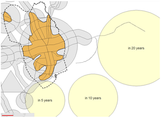
Thus, the total area for residential use will be at least 3,400 ha, 4,700 ha and 8,100 ha in 5, 10 and 20 years time. (All figures in this approach are very approximate and should only help to give a rough estimate).
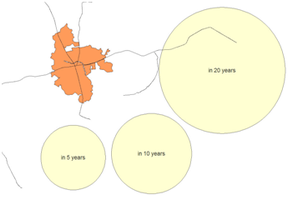
Decide on the best and most likely scenario and visualize the area required for this scenario.
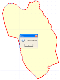
For comparison of the area, you can either select the planning area (as the only visible unit on screen) and assess its size with right-mouse > Measurement > Flood-fill measure:
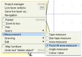
Or, you can draw a circle next to your planning area (with right-mouse > Drawing > Circle) and then measure the area of the circle (with same command as above).
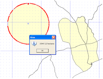
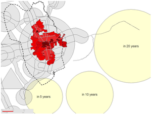
You now have an impression how much land will be required for the chosen scenario. This ‘area’ has to be ‘distributed’ in the planning area.
It is recommended to calculate and to display the areas of residential growth on your map. Use the formula:
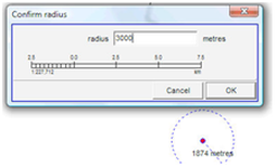
radius = sqrt( area (in ha) * 10,000 / 3.14 ).
At the example table above, that reads as:
In 5 years time: 3400 ha radius of 3300 m
In 10 years time: 4700 ha radius of 3900 m
In 20 years time: 8100 ha radius of 5100 m
You draw these circle of future land requirements: Right-mouse > Drawing > Circle > Point to a location outside the map as the centre point of the circle, and draw a certain distance > Confirm radius window: Enter radius (in meters) > OK
- - - - -
1. Define and draw exclusion zones, which are not suitable - or not recommendable - for any other than the specified use. They are not to form part of the land use pattern for urban planning in the Structure Plan:
Geological hazard areas,
Steep terrain,
Waterbodies,
Flooded areas or areas prone to flooding in one to ten / twenty year cycle,
Groundwater protection areas,
Flood prevention / control areas,
Military restricted areas,
etc
You can have these zones as separate layers or – better – merge them into one layer by collecting them individually, then one after the other copy to the same live layer, and save this in one file, which is the first version of the Structure Plan, e.g. Kasoa_structure_temp01.
- - - -
2. As development relies on development axes (‘corridors’), you have to draw major roads, both existing roads from road map and planned, new roads for road corridors in future. Both MTDP and Framework (see Chapter 7.4should guide you. You can start with the planned road layer for the Framework (step 2 of Chapter 7.4.3 but might need more details (and more roads).
You can copy-paste main existing roads from your road map into the new layer (e.g. Roads_planned). You can also draw new roads based on connection needs of newly developed parts in the planning area:
- Draw the road with the Line-tool from the toolbar left. In many areas, feel free to bring new ideas for the course of the roads.
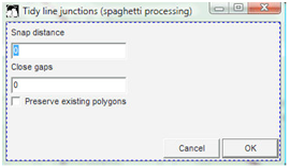
- If you intersect with existing roads, because your proposed road track is straighter than existing tracks with many bends, or you interconnect with an existing road network, you clean the topology by Cut, then Edit > Action > Snap vertex to nearest vertex (see Chapter 2.11) or – faster: - with the intersect option:
Selection Manger window > Select roads to be intersected with the Select-tool (at toolbar left) > Actions > Tidy > Tidy line junctions (spaghetti processing) > Tidy line junctions window: Snap distance: 0 > Close gaps: 0 > OK
When taking road proposals from existing road layer, delete all other road, then possibly connect road segments into one road and straighten it. Do not forget, this is a plan, not an engineering drawing for road construction.
Selection Manger window > Select roads to be handled with the Select-tool (at toolbar left) > Actions > Remove redundant line junction > Smoothen lines > Smoothen lines window: Tolerance: 10 (m) > OK
- - - - -
Remark for step 3ff: The operational, practical step of Structure Plan approximation(s) has not been established for land use planning at TCPD. Some steps have been taken out.
3. Have a draft concept, where to place the major kinds of land use (major planning zones).
Get a broad picture, i.e. a first draft map, with these general units by drawing them as polygons in this sequence:
Industry (if any)
Transport corridors and hubs (often predefined by the development corridors, see above)
Business and commerce (often along the main roads and corridors, or in centres or ‘hubs’)
Greens (including agricultural land, ecological reserves, ‘green belts’, gardens)
Residential
Other planning-specific areas might be included in this list on higher or lower priority.
At this stage, dont worry, if units are defined only 'generally', i.e. only with their general spatial delineation, and if some of the units overlap in this stage. It is common to have such a common ‘conflict’ over land use. This will be sorted out later in the process, both at the GIS and in participation with stakeholders and the community.
It might look similar to a Framework Plan, but these units are actual mapping units, not cartographic symbols like the circles, buffers, triangles of a Framework (see lt Chapter 7.4.1
- - - - -
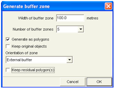
4. Buffer roads with individual buffer widths. For example, give a width of 100 m on both sides of main national highways, 50 m on other main trunk roads.
- 4.1 For such a differentiated buffering, you first create layers with different road classes. (For example, layers Kasoa_roads2buffer1 and Kasoa_roads2buffer2).
Draw 2-6 parallel buffers along a main road (see Chapter 3.1 for general buffering procedures).
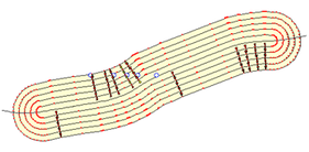
Follow instructions in Chapter 3.1.5 for clearing the many vertex points.
Assign general planning units to the buffers. You might have to cut units with the Cutter-tool and/or to combine them with the Join-tool from the toolbar left (before, snapping with the Snap-tool) and/or to make smooth transitions by editing vertex points of the polygon(s), followed by snapping.
- 4.2 For each of the road classes, join the buffer units with the Unite-file option: Main menu > Utilities > Vector utilities > Intersect/Unite files > Intersect lines and polygons window: Add file > Select all individual buffers > Tick ‘Find intersections’ > Tick ‘Tidy boundaries’ > Execute > Save result as > Save under temporary file name > Quit
- 4.3 After buffering, don’t forget to ‘clean’ the buffer layers: In live layer mode: Right-mouse > Live layer actions > Tidying > Tidy polygon topology > OK > Live layer actions > Tidying > Remove segments smaller than > OK > Remove segments smaller than window: 20 m > OK
- 4.4 Merge the different buffer class layers: Copy them all to live layer > With the Join-tool (at toolbar left), join all buffer polygons
- - - - -
5. Buffer rivers in a similar way, if they form flood protection areas.
- - - - -
6. In a similar way as explained above with the development corridors (buffering), proceed with development centres or hubs.
Create buffer circles around the centre points and combine them.
- - - - -
7. With exclusion zones (see step 1 above), industrial and commercial areas (see step 4 above), defined and all in one temporary layer (for example, Kasoa_structure_temp01), you assess the extension of the residential area.
Take the current land use map (see Chapter 7.2) and delete all non-residential areas. Thus, only low, medium and high density residential areas should show.
Combine these three different levels into one (with the Join-tool from the toolbar left, see Chapter 2.12).
Set this currently populated areas in comparison with the area required under the forecast (see above). Be aware, that quantitative definitions of ‘low, medium and high densities’ of these two assessments might be different.
Assign additional space around the residential area in direction of development according to the Framework. Have a display showing current residential areas, scenarios of future land requirements and Framework recommendations.
From there, you can draw the extensions of residential areas – in general terms. At this stage don’t worry about minor topographic ‘conflicts’ or ‘incompatibilities’.
By now, you have a picture of the residential area extension in the planning area.
- - - - -
8. Join this layer with the previously created (for example, Kasoa_structure_temp01) and merge them all by copying them to the live layer. Use style StructurePlan (see Annex 6.4 and Chapter 6.2.8 for the procedure to load it in your live layer)
- - - - -
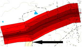
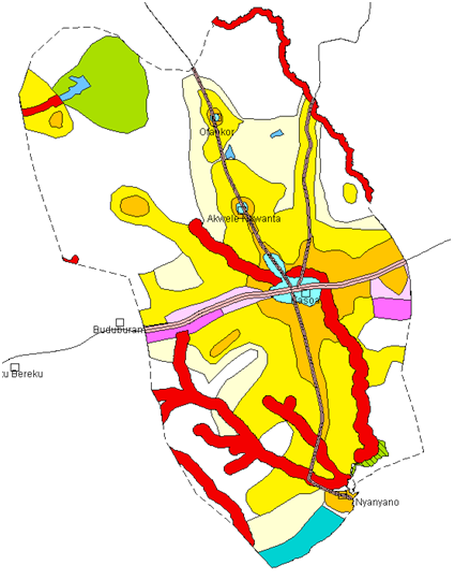
9. You might still have polygons overlap each other.
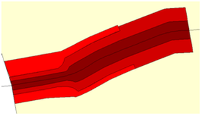
In the example below, the road buffers and the river buffer overlap and have to be clipped against each other (‘intersected’).
Main menu > Utilities > Vector utilities > Intersect/Unite files > Intersect lines and polygons window: Add file > Load layers, which overlap (select folder and file(s)) > Tick ‘Find intersections’ > Tick ‘Tidy boundaries’ with 0 m > Leave other options unticked >
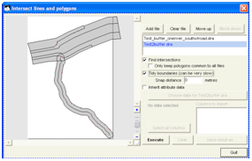
Execute > Save result as… > Specify temporary file name > Save > Quit
Load this temporary file
If some units disappear, you have obviously not snapped them properly. Snap all boundaries and repeat the process of intersecting the layers.
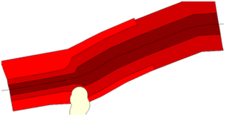
Be aware, that through this process you loose your display labels and styles. It is the easiest (but not shortest), to assign them again. Alternatively, you can use the seed facility (see Chapter 4.6).
- - - - -
10. Unless you did before, clip with the planning area layer by right-mouse > Live layer actions > Live layer actions window: Basic operations > Cut with file > OK > Cut with file window: Cutter file > Select folder and file name of planning area layer > OK (see also Chapter 3.6).
- - - - -
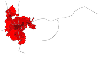
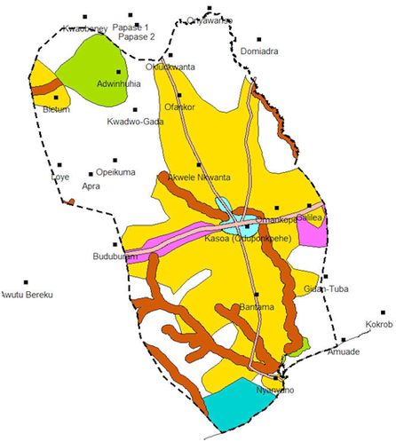
11. Save this layer in a file. It can look like this:
- - - - -
Remark for step 12ff: The operational, practical step of Structure Plan approximation(s) has not been established for land use planning at TCPD. Some steps have been taken out.
12. After this, get a more detailed description and definition of these planning zones, but not necessarily a better ground-delineation. I.e. refine the broad, general units of the previous steps to the structure plan classification (see Annex 6.4).
Load the classification (classes) for the final Structure Plan (style library StructurePlan, see Annex 6.4).
Copy the layer created in the previous steps (1-11) to a different file (e.g. Kasoa_structure_temp51). Have the land use map as a background (e.g. as a line map, with style Polys_AllTransp). You can also have the raster map or the orthophotos or a topographic map as background.
Zoom in to a slightly more detailed scale (screen scale of 2 – 0.5 km). Do not attempt to see all details. You will only loose the overview.
- - - - -
13. Use the Cutter-tool from the toolbar left to split the units. (See technical notes in Chapter 7.5.5, particularly part B).
- 13.1 Split the residential area(s) into low, medium and high density areas:
Low density housing area might be related to:
High income, upper class population (i.e. with high quality housing expectations) or
Poor environmental conditions (if infrastructure can not support sufficient human carrying capacity).
High density housing might be in:
Low income areas
Inner city areas
Vicinity to urban centres (with construction of multi-storey houses and CBD)
Create a good mix of low, medium and high density residential areas. Have an empiric approach, how large each unit can be (in peri urban areas some 500-1000 m, in central urban areas smaller, in rural areas larger).
- 13.2. Split business and commercial areas in functionality:
CBD in major towns
Formal business areas in towns, with offices, shopping malls, etc
Informal business areas, with local markets, mix with smallholder industrial activities like workshops etc
- 13.3. Split industrial areas according to their main function.
- - - - -
14. The next result can look like this:
Save this layer in a new file. It is recommended to use the letters 2ndapprox at the end of the file name (e.g. Kasoa_structure_2ndapprox).
- - - - -
15. You are now ready for the final delineation. This is an accurate delineation of all mapping units. You have to fine-tune the units according to:
Topography (rivers, mountains),
Adjacent land use zones,
Existing structures (buildings, roads).
It is important that delineation of planning units does not interfere with existing structures on the ground in a destructive way. The background information of the most recent orthophotos is therefore important.
You should zoom in to a screen scale of 250-500 m to see all details.
Incorporate all natural features, which wee mapped for the land use, such as rivers, mountains, lakes into this final Structure Plan.
Feel free to change units and boundaries. This is still possible in this stage.
You can also allocate areas of transition and mixed land use.
Topo maps (either scanned or digitized with contours, rivers etc). orthophotos and current land use (see Chapter 7.2 for land use mapping) are the most important background features on your display, when you ‘fine-tune’ the buffer units
You might have to ‘toggle’ between different display modes to get the best picture of the area. Make use of:
‘Blend’ raster images (orthophotos, scanned topo maps etc)
Set visibility to ‘Hide layer’
Set style of polygons to transparent, only display of polygon border (Style: Polys_AllTransp)
In already built-up areas it is often easy to ‘twist’ around existing structures, which can not be changed, i.e. established building, constructed roads, bridges, exclusion areas. You have to be in editing mode (live layer) with – preferably – a ‘transparent’ style for the layer.
Switch to transparent mode when editing: In live layer mode: Edit-tool (at toolbar left) > Click on any polygon > Polygon window: Styles > Edit project style set > Style set editor window: Style management > Import style set and overwrite > Choose style set window: Select Polys_AllTransp > OK > OK > OK
If you change the boundary between two land use zones (polygons), be aware that you have to change the boundary of each of these two polygons, and snap them together afterwards.
The best is to go through the entire planning area, from North to South, from West to East, photosheet by photosheet.
By now, you should have a good understanding of the entire area, of the terrain and of the existing structures on the ground. You now have a lot of data, i.e. map layers, that you can display and present the final Structure Plan.
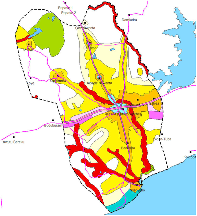
The sample map below demonstrates the basic features of a Structure Plan, here of the Kasoa planning area. The actual Structure Plan of this area considers more input parameters and is considerably larger and more complex, and has marginalia and legend (see Chapter 7.5.4).