A20.3 Excel: Lookup - LUPMISManual
Main menu:
- 0. Introduction
- 1. GIS handling
-
2. GIS data entry
- 2.1 Create new layer
- 2.2 Digitize line
- 2.3 Digitize point
- 2.4 Digitize polygon
- 2.5 Edit existing layer
- 2.6 Delete feature
- 2.7 Split line
- 2.8 Split polygon
- 2.9 Merge lines from different layers
- 2.10 Unite lines
- 2.11 Snap lines
- 2.12 Join polygons
- 2.13 Extend polygon
- 2.14 Insert island
- 2.15 Define unit surrounding islands
- 2.16 Create 'doughnut'
- 2.17 Fill 'doughnut' polygon
- 2.18 Fill polygon with 'holes'
- 2.19 Digitize parcels from sector layout
-
3. GIS operations
- 3.1 Create buffer
- 3.2 Create exclusion zone
- 3.3 Overlay units
- 3.4 Convert line to polygon
- 3.5 Derive statistics (area size, length)
- 3.6 Clip unit according to other unit
- 3.7 Create geographic grid
- 3.8 Move entire vector map
- 3.9 Move or copy individual features on a map
- 3.10 Adjust polygon to line
- 3.11 Convert points to polygon
- 3.12 Define by distance
- 3.13 Create multiple objects
- 3.14 Transfer styles from one layer to another
-
4. Attribute database
- 4.1 Start with database
- 4.2 Import database
- 4.3 Display database information
- 4.4 Enter attribute data
- 4.5 Attribute matrix of multiple layers
- 4.6 Seeds
- 4.7 Repair attribute data
- 4.8 Merge lines with attached database
- 4.9 Transfer attribute data from points to polygons
- 4.10 Copy styles, labels, attributes
-
5. Conversion of data
-
5.1 Points
- 5.1.1 Import list of points from text file
- 5.1.2 Import list of points from Excel file
- 5.1.3 Convert point coordinates between projections
- 5.1.4 Convert point coordinates from Ghana War Office (feet)
- 5.1.5 Convert point coordinates from Ghana Clark 1880 (feet)
- 5.1.6 Track with GPS
- 5.1.7 Download GPS track from Garmin
- 5.1.8 Download GPS track from PDA
- 5.1.9 Frequency analysis of points
- 5.2 Vector maps
- 5.3 Raster maps
-
5.4 Communication with other GIS programs
- 5.4.1 Import GIS data from SHP format
- 5.4.2 Import GIS data from E00 format
- 5.4.3 Import GIS data from AutoCAD
- 5.4.4 Export LUPMIS data to other programs
- 5.4.5 Export GIS to AutoCAD
- 5.4.6 Change a shape file to GPX
- 5.4.7 Transfer GIS data to other LUPMIS installations
- 5.4.8 Digitize lines in Google Earth
- 5.5 Terrain data
- 5.6 Export to tables
- 5.7 Density map
-
5.1 Points
-
6. Presentation
- 6.1 Labels
- 6.2 Styles and Symbols
- 6.3 Marginalia
- 6.4 Legend
- 6.5 Map template
- 6.6 Final print
- 6.7 Print to file
- 6.8 3D visualization
- 6.9 External display of features
- 6.10 Google
-
7. GIS for land use planning
- 7.1 Introduction to land use planning
- 7.2 Land use mapping for Structure Plan
- 7.3 Detail mapping for Local Plan
- 7.4 Framework
- 7.5 Structure Plan
- 7.6 Local Plan
- 7.7 Follow-up plans from Local Plan
- 7.8 Land evaluation
-
8. LUPMIS Tools
- 8.1 General
-
8.2 Drawing Tools
- 8.2.1 Overview
- 8.2.2 UPN
- 8.2.3 Streetname + housenumbers
- 8.2.4 Lines
- 8.2.5 Arcs
- 8.2.6 Polygons
- 8.2.7 Points
- 8.2.8 Cut line
- 8.2.9 Other Drawing Tools
- 8.2.10 Import
- 8.2.11 Projections + conversions
- 8.2.12 Format conversion
- 8.2.13 Other GIS Tools
- 8.2.14 Utilities
- 8.3 Printing Tools
- 8.4 Permit Tools
- 8.5 Census Tools
-
8.6 Revenue Tools
- 8.6.1 Overview
- 8.6.2 Entry of revenue data
- 8.6.3 Retrieval of revenue data
- 8.6.4 Revenue maps
- 8.6.5 Other revenue tools
- 8.7 Reports Tools
- 8.8 Project Tools
- 8.9 Settings
-
9. Databases
- 9.1 Permit Database
-
9.2 Plans
- 9.2.1 Accra
- 9.2.2 Kasoa
- 9.2.3 Dodowa
- 9.2.4 Sekondi-Takoradi
-
9.3 Census Database
-
9.4 Revenue Database
-
9.5 Report Database
-
9.6 Project Database
- 9.7 Address Database
-
Annexes 1-10
- A1. LUPMIS setup
- A2. Background to cartography/raster images
- A3. Glosssary
- A4. Troubleshooting
- A5. Styles
- A6. Classification for landuse mapping/planning
- A7. GIS utilities
- A8. Map projection parameters
- A9. Regions / Districts
- A 10. Standards
-
Annexes 11-20
- A11. LUPMIS distribution
- A12. Garmin GPS
- A13. Training
- A14. ArcView
- A15. Population statistics
- A16. Entry and display of survey data
- A17. External exercises
- A18. Programming
- A19. Paper sizes
- A20. Various IT advices
- A21. Site map and references
A20.3 Excel: Lookup
Level of expertise required for this Chapter: Intermediate
For report and table production, it might be necessary to link different tables from the GIS in a spreadsheet. Excel offers a range of 'lookup' functions: 'VLookup' (Vertical Lookup) is explained here.
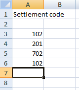
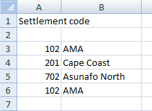
1. Situation: You have a spreadsheet with values, where you want to have the lookup values next to them:
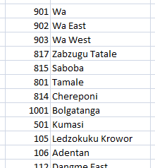
The reference table can look like below (example: District codes and names). See Chapter 5.6 ('Export tabular GIS data') for compiling this listing.
2. Sort this reference table: Select all values (2 columns) > Data > Sort > Sort by: Select left (reference value) column > Order: Smallest to Largest > OK
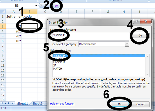
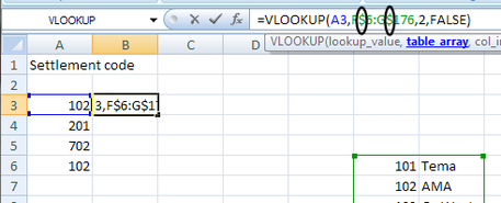
3. Link top cell: Select cell right of top first original cell [1 in screen shot below] > Press fx > In Search field: Type VLOOKUP [3] > Go [4] > Select VLOOKUP [5] > OK [6] >
> Lookup_value: Click in empty line next to 'Lookup_value' [1 in screen shot below] > Select top first cell [2] >
> Table_array: Click in empty line next to 'Table_array' [3] > Select entire entire array of reference set with 2 columns (which was just sorted) [4] >
> Col_index_num: In empty line next to 'Col_index_num': Enter '2' (for second column of this array) [5] >
> Range_lookup: In empty line next to 'Range_lookup': Enter 'false' [6] > OK [7]
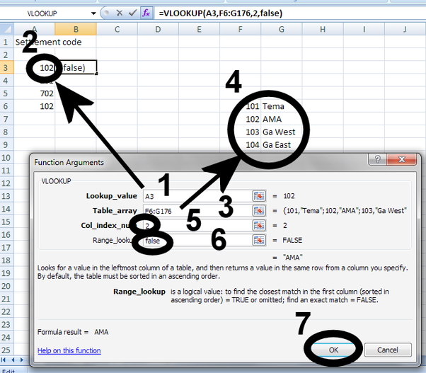
The first cell should get the reference value.
4. Insert $ (row fixer) to all row references in this first cell:
5. Copy this cell all the way down. Finished.
For Experts: If you have an empty reference, it will return #N/A. To avoid this and have an empty (text) field, you have to modify the reference formula to: